Simple pipeline

A simple pipeline expliciting with

• reading some spectral data

• plotting the data

• plotting data with additional informative vertical band

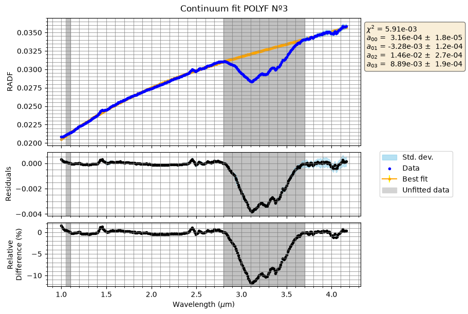
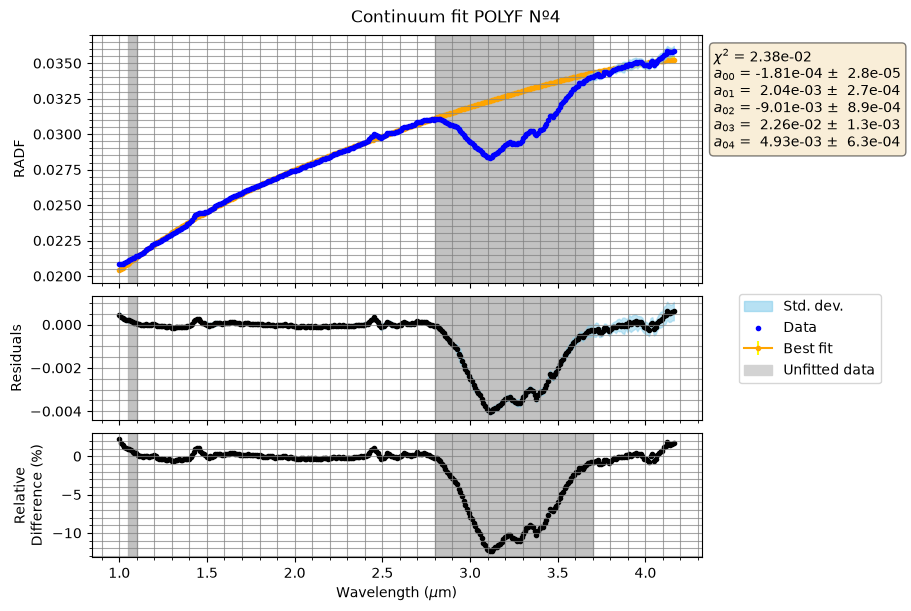
• fitting the data’s continuum

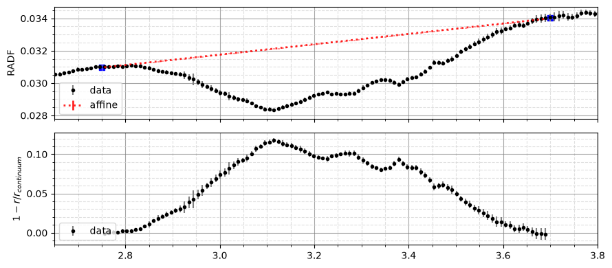
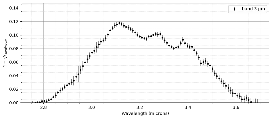
• extracting a band from that data

• running a simple fit on the extracted spectral band

import numpy as np
from specmodels.specmodels_base import SpecModel
import specmodels.specmodels_functions as sf

import os

print(os.getcwd())
print(os.path.dirname(os.path.realpath("./raponi_2020_67p_virtis_mir.txt")))

/workspace/cxlfeller/specmodels/pipelines/simple
/workspace/cxlfeller/specmodels/pipelines/simple

# Plot 67P data
data = SpecModel(
    data="./raponi_2020_67p_virtis_mir.txt",
    label="67P (Raponi+2020)",
    ylabel="RADF",
    interpolation_order=5,
)

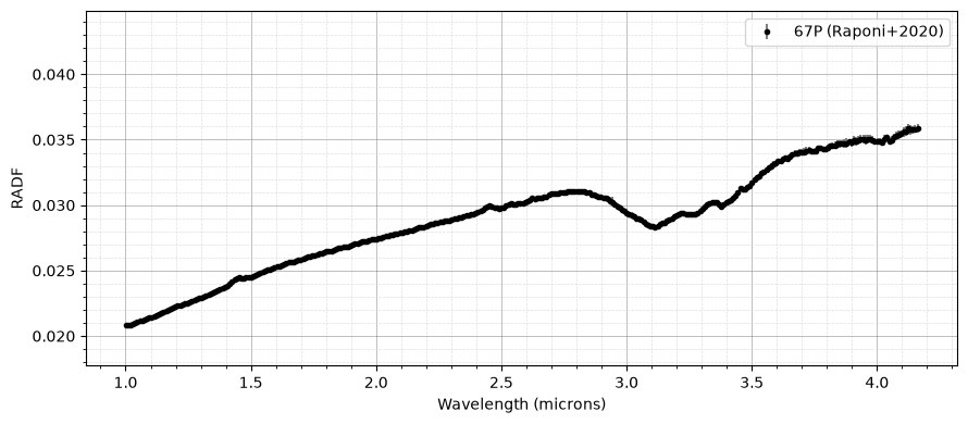
# Regular plot
_ = data.base_plot()

# Define rectangle parameters
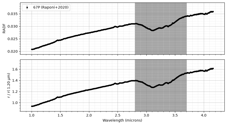
rect_params = [
    dict(
        xy=(2.80, 0.0),
        width=0.90,
        height=5.0,
        edgecolor="grey",
        facecolor="grey",
        alpha=0.7,
    ),
]

_ = data.base_plot_norm(wl_ref=1.2, rects=rect_params)

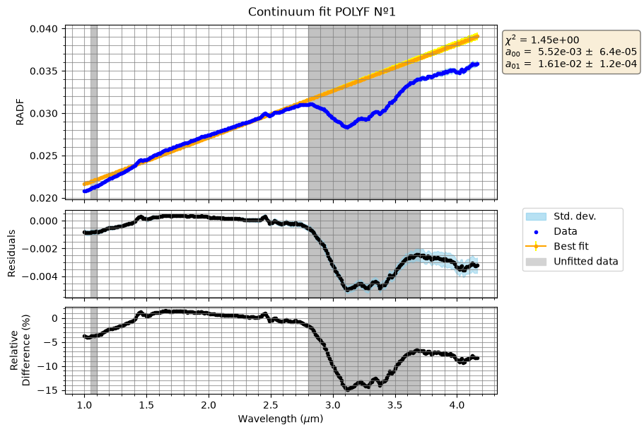
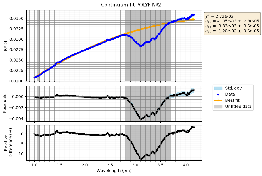
# Define a set of spectral features to ignore in the fitting
# 1.05 -> 1.10
# 2.80 -> 3.70
mask = np.array([[1.05, 1.10], [2.8, 3.7]], dtype=np.float64)
# Reset the initial continuum fit with the added information
data.continuum_update_fits(order_max=4, mask=mask)
# Re-plot
_ = data.continuum_plt_fit(mask=mask)

band_3 = data.rectify_extract_band(
    wrange=np.array([2.75, 3.7]),
    dlt=np.array([[0.05, 0.05], [0.05, 0.05]]),
    label="band 3 µm",
)

_ = band_3.base_plot()

# Simple gaussian fit
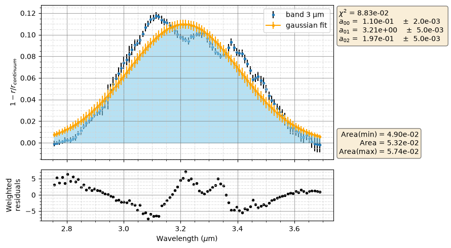
rd, _, _ = band_3.fit_simple(sf.gaussian, area=True)

# Run fits with multiple gaussians
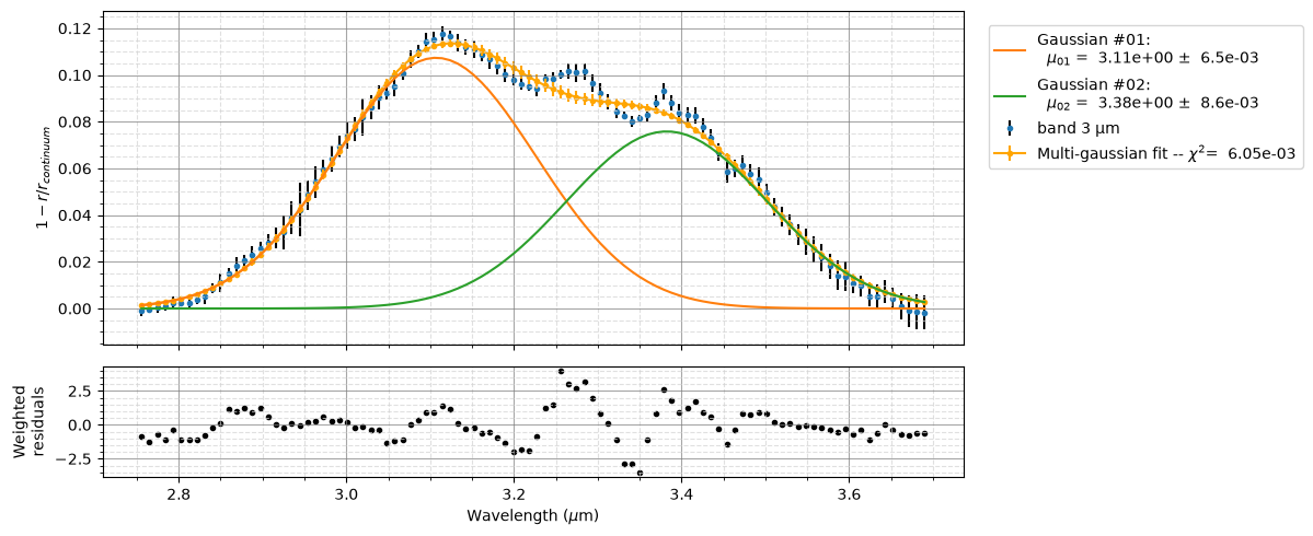
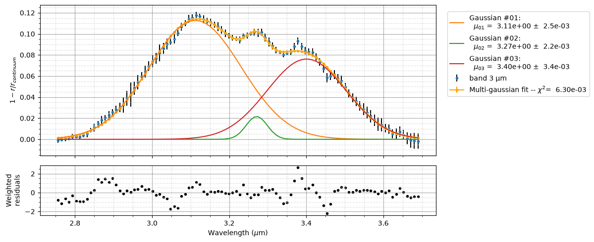
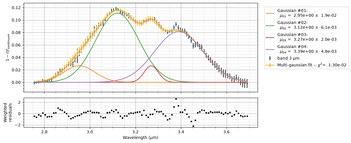
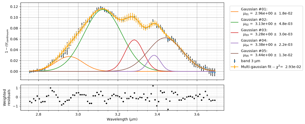
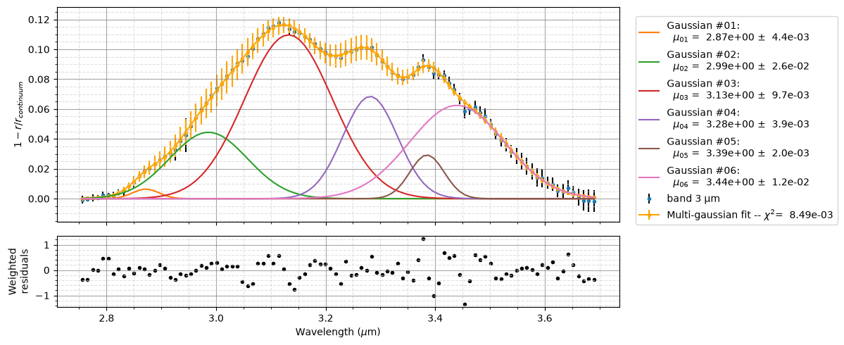
mgauss_dvals = band_3.mgauss_nfits(ngaussians=list(range(2, 7)))

# Plot multifit results with individual gaussians
for dfit in mgauss_dvals:
    _, _ = band_3.mgaussfit_plot(dfit)

---

#EOF