Hapke models
Dr. Bruce Hapke has published his theory over several papers, accounting for improvements and modifications [1, 5, 7, 8, 9, 10]. The model assumes that particles are larger than the wavelength, irregular in shape, randomly oriented and positioned. We will present here various reflectance models in order to progressively introduce the different components of the IMSA model.
Reflectance of dark surfaces observed at high phase angles
A model “0” of the reflectance in the frame of the RTE actually corresponds to the reflectance derived by Lommel, which only considers single scattering in media with a albedo lower than 50%. Such a reflectance would actually describe a dark and smooth surface observed at large phase angles (beyond \(10^{\circ}\)). As presented in Hapke [1], its expression is:
where \(\mu_{0}\) and \(\mu\) are respectively the cosine of the incidence and emergence angles, and p(\(\alpha\)) is referred to as the single particle phase function (sppf). A simple analytical expression of the average sppf of the medium is not possible to derive for irregularly shaped particles. One then relies on the empirical model of Henyey and Greenstein [11], which describes a direction-favoured reflection. This phase function can be used to describe a situation where a particle scatters preferably either towards the source or towards the observer (single-lobed function, noted \(p_{HG,1}\)), or a case where a particle scatters differently towards the source and towards the observer (two-lobed function, noted \(p_{HG,2}\)). Their respective expressions are as follow:
Where g is the asymmetric scattering factor (hereafter noted \(g_{scat}\)) and c is the mixing angle between the two lobes (i.e. their respective proportion). The asymmetric factor belongs to the \(]-1,1[\) interval: when \(g_{scat}\) is negative, the phase function describes a particle scattering preferentially towards the source (the particle is then said to be backward-scattering) and in the opposite case, the particle scatters preferentially towards the observer (the particle is then said to be forward-scattering). This property is well illustrated in Fig. 4, where the peak of the lobe is similarly reached either at \(0^{\circ}\) or at \(180^{\circ}\).
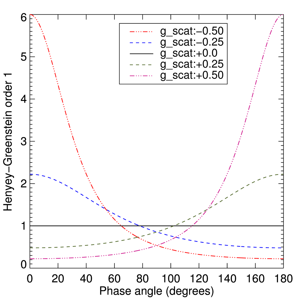
Fig. 4 Plots of the \(p_{HG,1}\) using various values of the asymmetric scattering factor \(g_{scat}\).
In the general case, two peaks of different widths would be reached at either end.
Reflectance of non-opaque surfaces: the IMSA and AMSA models
While the consideration of extinction and single scattering only bring to the Lommel-Seeliger reflectance, the inclusion of the multiple-scattering adds another term, which describes a situation where the regolith’s particles are less absorbing and some photons are scattered multiple times before being scattered in the direction of the detector. Similarly, the previous expression of the reflectance becomes:
where \(M_{scat}\) is the multiple scattering term. In the descriptions of the model prior to Hapke [9], the multiple scattering contribution is assumed to be isotropic, and while the single-scattering term is calculated exactly in the RTE, the multiple scattering term is approximated using the two-streams method [12] and has then for expression:
Where the H function corresponds here to a second-order approximation of the Ambartsumian-Chandrasekhar function [2, 13]. The H function describes the incoherent isotropic scattering of the radiance in a semi-infinite medium of infinitesimal layers, either toward the upper layer or towards the lower layer. With this expression of the \(M_{scat}\) component, the model described by eq. (6) is referred to as the Isotropical Multiple Scattering Approximation (or IMSA). However, in Hapke [9], the expression of the multiple scattering was revised to consider the case of anisotropic multiple scattering and so becomes:
Where in the formula above, the expressions of P( \(\mu\) ), P( \(\mu_{0}\) ) and P are are defined as:
In a frame of the regolith’s description as a semi-infinite medium of infinitesimal layers, the multiple scattering term \(M_{scat}\) corresponds to the combination of the scatterings of the radiance by the volume element towards the lower layer and towards the upper layer, and therefore each depends on the particle phase function. In particular, when the volume element is illuminated from a direction that makes an angle i with the normal to the surface, the average scattered radiance toward the lower hemisphere is denoted as P( \(\mu_{0}\) ). Similarly, when the same volume element is uniformly illuminated from the lower hemisphere, the average scattered radiance towards the direction making an angle e with the normal to the surface is denoted P( \(\mu\) ). Finally, of all of the radiance scattered upwards by the entire lower hemisphere, the volume element scatters back in average an amount denoted as P. Using this description of the multiple scattering, the model described by eq. (6) is referred to as the Anisotropical Multiple Scattering Approximation (AMSA).
As shown in Hapke [9], those integrals can be expanded as a serie of Legendre polynomials depending on the chosen expression of the average particle phase function, and can be so evaluated.
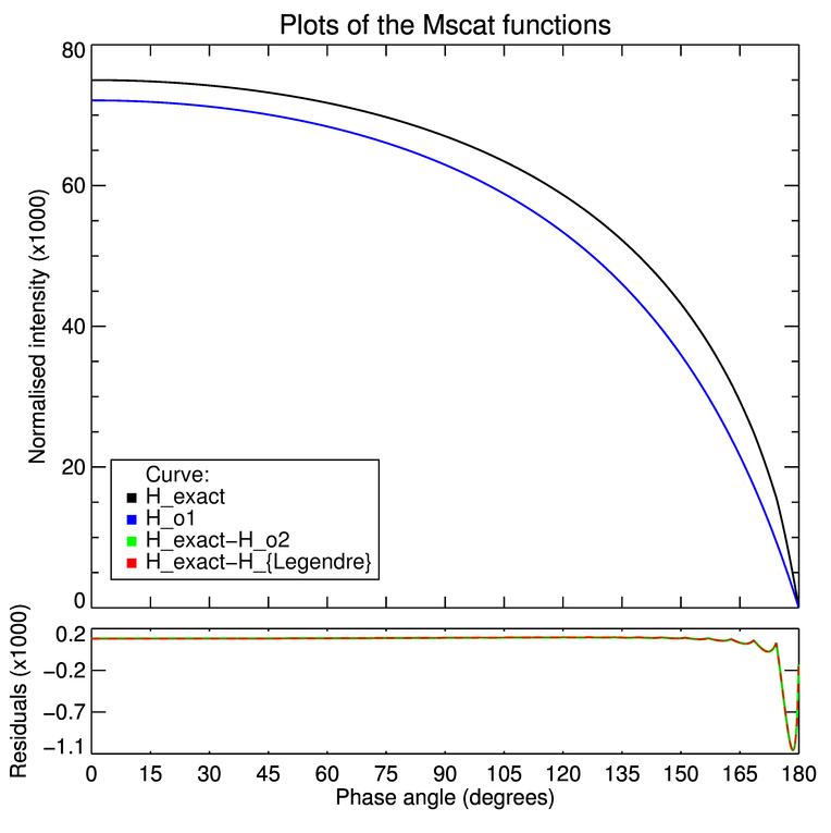
Fig. 5 Plots of the different expressions of the multiple scattering function for an albedo of 10%: (upper plot) \(H_{exact}\) refers to the values tabulated in Chandrasekhar [2], Nath Das and Bera [14], \(H_{o1}\) refers to the first order approximation of the function [5]. For clarity, only the residues of the second order approximation and the Legendre polynomial expansion with the exact values are plotted (bottom plot).
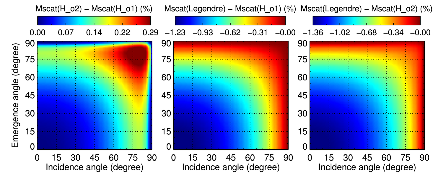
Fig. 6 Mapping in the (i,e) space of the difference in reflectance given the three possible expressions of \(M_{scat}\), using an \(w_{ssa}\) of 3.4% and assuming an isotropic sppf (p(g)=1).
Hence, we gathered from the papers published by Dr. Hapke three expressions describing the multiple scattering contribution to the overall reflectance of the regolith surface. As shown in Hapke [9], we illustrate here in Fig. 5 and Fig. 6 the minute difference between those three expressions.
In the upper plot of Fig. 5, we drew the variations of the \(M_{scat}\) function for an albedo of 10% based on the values tabulated in Chandrasekhar [2], Nath Das and Bera [14] for the H-function, and its first-order approximation given notably in Hapke et al. [5]. In the lower plot, we drew the differences of the exact values with the second order approximation and the polynomial expansion (see for instance Hapke [9]). The shallowness of the differences is well illustrated by the fact that the scale of the ordinates axis has been multiplied by a thousand. While, as illustrated in Hapke [9], there is a notable difference between the exact solution and the first-order approximation, in the \(0^{\circ}̀\) to \(90^{\circ}̀\) range (in which OSIRIS observations were taken), there is almost no difference between the exact solution, the second-order approximation and the Legendre polynomial.
This observation is further verified in Fig. 6, where we drew in the (i,*e*) space the difference between the Hapke-derived reflectances of a non-opaque isotropically scattering medium, whose associated single scattering albedo is of 10%, using the tabulated values of the H-function, and the different approximations used by Dr. Hapke. In those mappings, we verify that at large incidence angle (i \(\geq~75^{\circ}̀\)), using the first-order approximation would lead at worst to a 0.0045% difference, while for the second-order approximation and the Legendre expansion, it leads to a 0.0000065% difference at worst.
As a conclusion, those figures illustrate the minuteness of the differences between those different expressions. Further practical considerations if the implementation of a non optimized CPU-oriented version of the Hapke model pushed us to restrict ourselves here to the use of the expression of the multiple scattering postulated in Eq. (8). Indeed, that expression was about two orders of a magnitude quicker to compute over hundreds of thousands of data-points than the Legendre polynomials expansion.
Reflectance at small phase angles: inclusion of the opposition effect
In the sections above, as hinted, the models describe a smooth regolith’s reflectance observed at phase angles higher than :math:̀ sim 10^{circ}`. Indeed, at low phase angles, the reflectance of a rough particulate surface increases suddenly in a non-linear manner. This surge is named the opposition effect as it appears when objects of the solar system are at an astronomical opposition: when the sun, the earth and the object are aligned. The first historical report of the observation of the opposition effect is the florid description of the sixteenth-century Florentine sculptor Benvenuto Cellini of the extraordinary halo around the shadow of his head on the grass. Yet, the opposition effect is a common property of particulate media such as laboratory powders [15, 16], the Moon’s regolith [17], asteroids [18, 19], the disks of Saturn [20], and also satellites of the outer planets [21].
This sudden increase of the reflectance at small phase angles can be due to one of two phenomenons, or to their combination. Those two phenomenons are the shadow-hiding opposition effect (or SHOE) and the coherent-backscattering opposition effect (or CBOE).
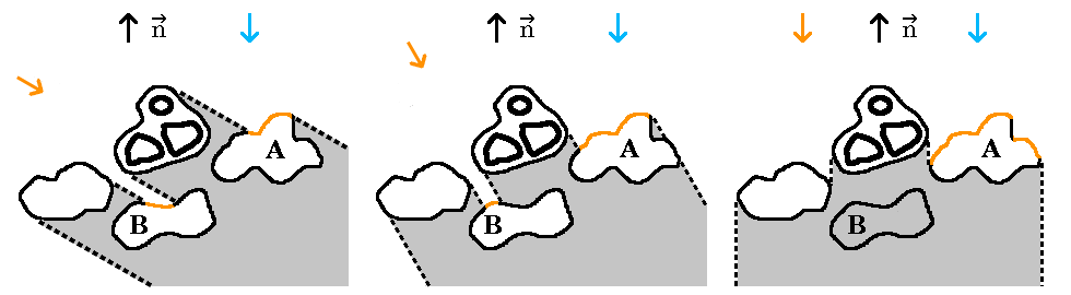
Fig. 7 The shadow hiding opposition effect comes from the variation of the particle’ surface illuminated by the source and the growing absence of visible shadows from particles upon other directly visible one. The vector \(\vec{n}\) denotes the normal to the overvall surface. The gold and blue arrows denote the respective directions from the sun and towards the observer.
The shadow hiding opposition effect is simply the apparent disappearance of the shadows when the phase angle decreases towards \(0^{\circ}\). The SHOE occurs in any particulate medium in which grains are larger than the wavelength, so that grains cast shadows upon the grains located below them. While at large phase angles, some grains are masked in parts or wholly (grain A, left cartoon of Fig. 7, at small phase angles, the shadows are behind the objects that cast them and all the visible surface of the medium is illuminated. The radiative transfer equation does not account for the SHOE, and it is adjuncted in a ad-hoc manner in reflectance models [15, 22, 23, 24]. The analytical expression of the SHOE is used as an enhancing factor to the particle phase function, we report here the approximation of its expression given in Hapke [1]:
where, \(B_{SH,0}\) is the amplitude of the SHOE and \(h_{SH}\) its width. The amplitude is defined as the ratio of the scattering coefficient (S) close to the surface to the total amount of scattered light by the particle at zero phase angle . Meanwhile, the width of the SHOE is related to the particle’s volumic extinction coefficient (E), the average particle size (<a>) and the filling factor of the medium (φ) in [1, 9]. Their respective expressions are:
In this description, \(B_{SH,0}\) varies between 0 and 1 and \(h_{SH}\) ranges from 0. to 0.15. Yet Hapke [25] notes that for particles with a mean grain size less than 20 microns, the SHOE is particularly marked (for reference, most of the particle clusters captured by COSIMA have a height lesser than a 100 \(\mu\) m, according to Langevin et al. [26]). Around this particular size, the electrostatic and Van der Walls forces takes precedence over the gravitational forces, and this leads to the formation of complex structures referred to as fairy castle [15]. Room is left in the model [1] to interpret values of \(B_{SH,0}\) above 1 as a consequence of a particle being large and complex enough that its sub-structures cast shadows on themselves, meaning that the individual particle phase functions of the sub-structures would have their own SHOE.
The coherent-backscattering opposition effect appears due to the constructive interference of light waves as they emerge from the medium after having been scattered multiple times within or/and in-between the particles. The CBOE was initially discussed in Watson [27] and was first observed in a scattering experiment by a particulate medium in Kuga and Ishimaru [28]. The phenomenon has since been, and persists to be, the subject of theoretical and experimental investigations [16, 29, 30, 31, 32, 33, 34].
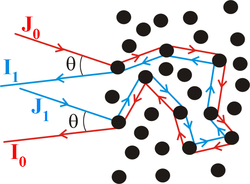
Fig. 8 In the frame of the far-field approximation, at low phase angles (when \(\theta~\sim~0^{\circ}\), multiple scattering within and between particles can induce a optical phase difference so that, upon emerging, the light waves scattered towards the observer (\(I_{0}\) and \(I_{1}\), in the cartoon above)} interfer coherently. Credits: wikimedia.org.}
The principle of the CBOE is illustrated in Fig. 8:
1. the wavefront (\(I_{0}\), \(I_{1}\)) incident on a particulate medium encounters scatterers;
2. the wavefront is then scattered within the particles, and in-between them (i.e. further deeper within the medium). Among the two parts, a portion of it will be scattered back towards the surface. Assuming the surface is lit homogeneously, for every possible path tread in one direction, part of the wavefront will travel it in the reverse direction;
reaching the surface, a portion of the wavefront is scattered towards the observer.
Hence, for the two portions of the wavefront which are scattered towards the observer (directly and after multiple scatterings), there is no difference in the optical path, therefore each of those portions may constructively interfere and the total of their respective intensities then quadruples. Thus bringing a surge in reflectance at low phase angles. This conclusion is reached under the assumption that the medium is not too absorbent: that the single scattering is large enough so the multiple scattering contribution is substantive enough with respect to the modulated particle phase function. The reader is here cautioned not to assume that multiple scattering is absent from a dark surface: the very opposite was shown for lunar measurements with normal albedos as low as 10% [35] as well as within mixture of magnesium oxides and dark coal powders [36]. For that reason, in the frame of the Hapke theory, the coherent backscattering is modeled as a property for the whole of the medium and is implemented within the reflectance model as a enhancing factor of the single particle phase function and of the multiple-scattering term.
Several analytical approximations are used in the Hapke theory to describe the coherent-backscattering modulation, which is added to the reflectance model in a ad-hoc manner. We retain here the original formulation of Akkermans et al. [37], and one formulation of Hapke [1]. The analytical expression developped by Akkermans using the notation of Hapke, is according to Shkuratov et al. [38]:
Where \(B_{CB,0}\) is the amplitude of the CBOE, \(h_{CB}\) its width, \(\lambda\) the wavelength, \(\Lambda\) is the average extinction length of the volume element. The analytical approximation formulated in Hapke [1] has for expression:
As hinted above, in the frame of the IMSA model [9], the coherent-backscattering is applied as a modulation of the whole reflectance, whose expression then becomes: