Introduction
This module provides tools to read, generate, visualize and fit photometric data. It will shortly be only limited to the Hapke photometric model, but be extended to other models afterwards.
Notions of photometry
A - Irradiance, radiance and fluxes
Going all the way back to the Maxwell-Lorentz equations, given a EM-waves source at an infinite distance, one defines the associated Poynting vector as the local energy flux per unit area per unit of time crossing a defined surface element at a point in space (in W/m^2/s).
The irradiance (J, W/m^2) of that is then defined as the average of the Poynting vector crossing a unit area perpendicular to the propagation direction of the EM-wave per unit of time.
That definition only stands in the case of a collimated beam. Opposingly, for an uncollimated beam propagating along a vector Ω, the time average of the Poynting vector traveling into the unit of solid angle around Ω is called the radiance (I, W/m^2/sr).
Performing measurements in a laboratory, one will usuall measure the radiance scattered in different directions by a surface sample illuminated with a collimated beam, to derive its properties. We note here, that some laboratory instruments (e.g. FTIRs) do measure the radiance for a surface illuminated with an uncollimated beam, but this case will not be covered here presently. For celestial bodies, one assumes that the investigated planetary surface is far away from the Sun to assume that the illumination is collimated.
B - Viewing geometry
Any observation of a surface can be described geometrically according to three angles: the incidence, the emergence and the azimuth angles. Together these angles define a viewing geometry.
Let SE be a surface element of a closed object and N a vector normal to SE pointing outwards, emerging from the surface at a point O. Let LS and Ob be respectively a distinct point-like light-source illuminating SE and an distinct observer of the surface. The plane containing both N and the direction vector from O to LS is known as the incidence plane (IP), and within that plane the angle between both vectors is known as the incidence angle (noted i). The plane containing both N and the direction vector from O to Ob is known as the emergence plane (EP), and within that plane the angle between both vectors is known as the emergence angle (noted e). Finally, the angle between IP and EP is known as the azimuth angle (noted φ).
Out of these three angles, a fourth angle is defined as the separation between the two direction vectors LS -> O and O -> Ob on the unitary sphere centered around O.
With the incidence, emergence, azimuth, and phase angles being noted as i, e, φ, g, Fig. 1 explicits the viewing geometry of a surface:
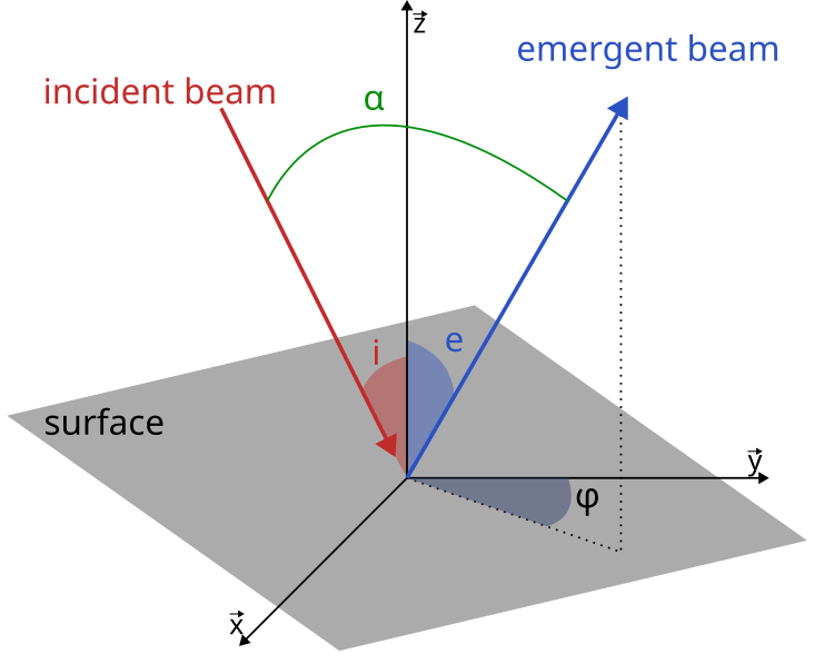
Fig. 1 Diagram illustrating the four angles defining a viewing geometry: the incidence (i), the emergence (e), the azimuth (φ) and the phase (α). CREDITS: Robin Sultana.
Inbetween the incidence, emergence, azimuth, and phase angles, the following relation stands:
This trigonometric definition implies a degeneracy of the phase angle, which is illustrated in Fig. 2, in which each diagram depicts a surface plot of g as a function of the couple (i,e) for a given value of the azimuth angle.
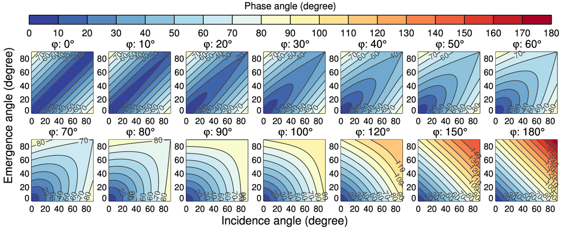
Fig. 2 Plots illustrating the multiplicity of similar observational configurations for a given phase angle value.
This degeneracy has for implication that several reflectance values associated with different sets of incident and emergence angles are identified with the same phase or azimuthal angle value, which will be illustrated later on in this documentation.
C - Reflectance(s)
For a given illuminated surface, the radiance is proportional to the irradiance, and their ratio, noted r, is called bidirectional reflectance. It is formally defined in Hapke [1] as:
The bidirectional reflectance r(i,e,g) is the ratio of the radiance scattered from the surface of a medium into a given direction to the collimated power incident per unit area perpendicular to the direction of incidence.
Thus \(r(i,e,g) = I(Ω) / J\).
We note here that the term reflectance is sometimes used inappropriately, as is, without the specific characterization. As in Hapke [1], and following Nicodemus+1970’s definitions, the term reflectance hereafter refers to the bidirectional reflectance. In fact, three other physical quantities derive from the bidirectional reflectance: - the bidirectional-reflectance distribution function (BRDF) - the reflectance factor (REFF) - the radiance factor (RADF, or I/F)
The BRDF is defined as the ratio between the radiance scattered by an investigated surface (\(J\cdot r(i,e,g)\)) and the collimated incident radiance per unit of surface area (\(J\cdot cos(i)\)). Thus:
The REFF is defined as the ratio of the same scattered radiance (\(J\cdot r(i,e,g)\)) to that of the radiance scattered by a corresponding Lambertian surface illuminated under an incident angle i (\(r_{L} = \cos\left(i\right)\cdot J /\pi\)), i.e. a perfectly diffuse surface. Thus:
Lastly, the RADF is defined as the ratio of the scattered radiance to that of the Lambertian surface’s illuminated normally. Thus:
The RADF quantity is also often noted as I/F, where F refers to the irradiance quantity defined by Chandrasekhar [2] as \(J /\pi\).
D - Radiative transfer Equation
The radiative transfer equation was derived in Chandrasekhar [2], and is notably used to model a planetary surface’s reflectance and to study planetary atmospheres [3, 4]. Considering Fig. 3, let there be a detector with a sensitive area \(\Delta a\) and intercepting a surface element within the solid angle \(\Delta w\). Let there also be an increment of volume \(dV = r^2dr\Delta w\) located at a depth z below the apparent surface and a distance r from the detector. This volume element is irradiated by the sunlight at the rate of J Watts per square meters, and it radiates I Watts per square meters along the solid angle \(\Omega\), the direction of the solid angle \(\Delta w\). Furthermore, let E, S and H be respectively the extinction, scattering and emission coefficients associated with this volume of regolith. The three contributions to the power received by the detector from \(dV\) are:
1. the radiation from the source (i.e. the Sun) that has been scattered once by the particles in \(dV\) along \(\Omega\);
the radiation thermally emitted by the particles in \(dV\) along \(\Omega\);
3. the radiation that has been emitted or scattered at least once, impinging on the particles in \(dV\) which scatter it along \(\Omega\).
When emerging from this volume element, the radiation is exponentially attenuated as it traverses the regolith and reaches the surface at a distance R from the detector. Hence the power budget is as follows:
Where G is angular scattering coefficient associated with this volume of superficial surface, B(T) is the Planck’s blackbody law and J the power directly incident to the volume dV (e.g. the solar irradiance).
As we consider hereafter only the case of detectors sensible to wavelengths ranges from the near-ultraviolet to near-infrared (i.e. 250 – 1000 nm), and assuming that the particles of the optically thick regolith are fundamental scattering units, we then define the average single scattering albedo w<sub>ssa</sub> as S/E and the average particle scattering function p(g) as G(g)/S. Hence the RTE becomes:
When solving this equation, one finally obtains a proportionality relation between the irradiance J and the radiance I, which defines the reflectance of the regolith using the RTE. In the coming section, we will present the Hapke canonical models of reflectance and parameters. The reader is referred to Hapke [1], Hapke et al. [5], Hapke [6] for detailed derivations.
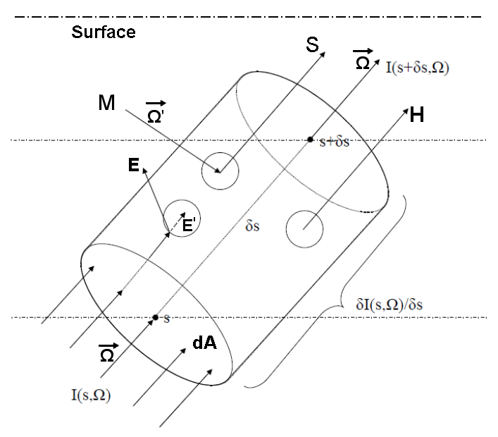
Fig. 3 Description of the radiative transfer equation, schematic of the changes in radiance as it traverses the cylindrical volume \(\delta s dA\). The elementary variation between the incoming radiance at depth s and the emergent radiance at depth \(s+\delta s\) along the direction \(\vec{\Omega}\) is equal to the radiance extinguished (through scattering E and absorption E’) and to the thermal emission (H) and the total radiance (incoming from the directions \(\vec{\Omega}\) and \(\vec{\Omega'}\) scattered in the direction \(\vec{\Omega}\). Adapted from Hapke [1].